Assumptions in the model :
There should be a linear relationship between dependent (response) variable and independent (predictor) variable(s).
If we fit a linear model to a non-linear, the regression model would not capture the trend mathematically, thus resulting in an inefficient model. Also this will result in erroneous prediction on out of sample data
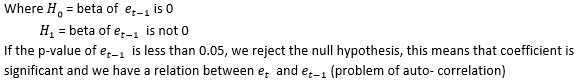
There should be no relationship between the residuals (error) terms. Absence of this phenomenon is called Auto Correlation.
The presence of correlation in error terms reduces model’s accuracy. This usually occurs in time series model. If the error terms are correlated, it underestimates the true standard error.
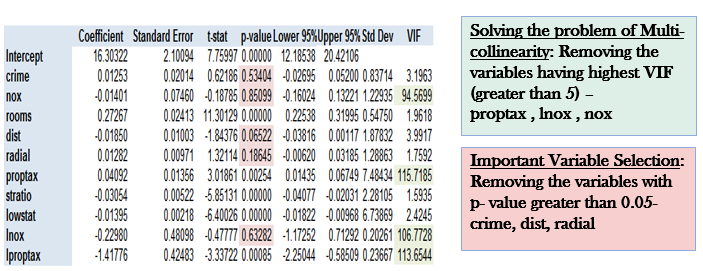
The independent variables should not be correlated. Absence of this phenomenon is called Multi-collinearity.
When predictors are correlated, the estimated regression coefficient of a correlated variable depends on the other predictor available in the model.
The error terms must have a constant variance. The presence of non-constant variance is called heteroscedasticity.
When this phenomenon occurs, the confidence interval for out of sample prediction tends to be unrealistically wide or narrow.
The error terms must me normally distributed.
Step 1: Removing multi-collinearity and important variable selection –
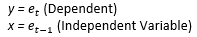
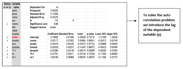
Step 2: Checking and Removing the problem of Auto correlation:
At first we calculate the residual error terms and the lag of residual error terms:
We need to check mathematically if correlation is present between error terms by running a regression with –
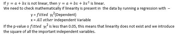
Step 3: Checking and achieving Linearity in the data:
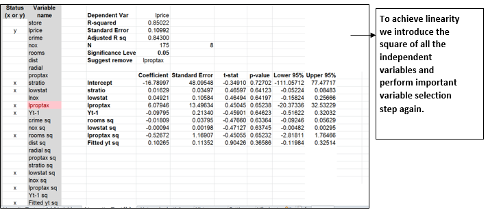
Step 4: To check if the data is homoscedastic or Heteroscedastic:
Heteroscedasticity is the problem of having a non – constant variance.
We perform a chi-square test to check if constant variance is present or not, where we compare chi-square statistic with chi- square critical.
Chi – square statistic – N* R square
Chi – square critical – chisq.inv function
If chi-square statistic is greater than chi- square critical then it is homoscedastic, otherwise Heteroscedastic.
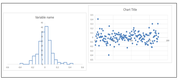
Step 5: Sanity Check:
For this test we would plot the values of all the error terms using Histogram and the Scatter plot.
If the histogram appears to be bell- shaped, it means that the error terms follow a Normal Distribution.